Example: Yagi-Uda Antenna Made Out of Silicon particles.

In this example, we will simulate a Yagi-Uda antenna made out of small silicon spheres (like in Krasnok et al., Opt. Express 20, 20599-20604 (2012), click here for more information). For this, we will create a linear structure of small particles as follows:

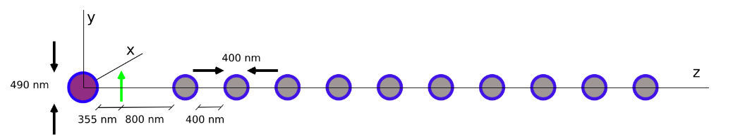
Note that the spacings described below have to be understood as center-to center spacing. At the origin, we place a silicon sphere with a radius of 245nm called the reflector. After a bigger spacing of 245nm + 355nm + 800nm + 200nm = 2600 nm within which we will place the emitter (an oscillating dipole source aligned along the y-axis) at a distance of 600 nm from the origin, we align 10 silicon spheres, called directors, on the z-axis and with a radius of 200nm, (center to center spacing: 800nm). We will then compute the emission pattern of this structure, in order to investigate the directionality of this antenna.

We suppose that you already know the example of the PS sphere. So if you haven't had a look to it before, read it first. If you want to know about the electric and magnetic CEMD problem, have a look at the theory as well.

If you want to run this example, copy it or download it from the GitHub repository (example_yagi_uda.jl) and run it using

julia example_yagi_uda.jl

Setting the Structure

We will first start to model the structure of the antenna in an array 'r' containing the positions of each of its components. But first, we need to import some libraries.

#imports
using CoupledElectricMagneticDipoles
using PyCall
using LaTeXStrings
using LinearAlgebra
@pyimport matplotlib.pyplot as plt

Then, we can set the parameters (sizes) of the antenna and build the structure.

##################### Parameters ########################################
#radius of the sphere (in μm)
a_refl=0.245 #reflector radius
a_dir=0.200 #director radius
N_dir=10 #number of directors
#dielectric constant of the particle
eps=12
#wavelength (in μm) 
lambda=1.550
##########################################################################

#setting the structure
#creates an array to contain the positions
r=zeros(N_dir+1,3)

#spacing between reflector and first director
spacing_ref_dir=a_refl+0.355+0.800+a_dir
#spacing between directors
spacing_dirs=4*a_dir

#sets the position of the directors (reflector is at the origin)
for i=2:N_dir+1
    r[i,3]=spacing_ref_dir+(i-2)*spacing_dirs
end

#creates an array containing the radius of each sphere
as=a_dir*ones(N_dir+1)
as[1]=a_refl

Modelling silicon particles

Now that we set the position of each of the antenna's components, we need to model their optical response. To do this, let's open a small parenthesis and try to model a sphere with a radius of 0.230 μm using only one electric and magnetic dipole per particle (no discretization like in the PS sphere example). For this, we set the electric and magnetic polarizabilities of the particles to be proportional to the two first Mie coefficients $a_1$ and $b_1$. For this, we use the MieCoeff module to get the Mie coefficients and to compare the scattering efficiency $Q_sca$ of the sphere computed with only the first Mie coefficient and the truncated series (cut after 20 terms).

#------------------modelling silicon particles---------------
#parameter
lambdas=LinRange(1.200,1.600,100)
knorms=2*pi./lambdas
a=0.230
ka = knorms*a
eps=12
#scattering cross sections
mie_sca=MieCoeff.mie_scattering.(ka,eps,1,cutoff=20)
dipole_sca=(6*pi)./knorms.^2 .*(abs2.(MieCoeff.mie_an.(ka, eps, 1, n=1)).+abs2.(MieCoeff.mie_bn.(ka, eps, 1, n=1)))
#plotting
fig1,ax1=plt.subplots()
ax1.set_xlabel(L"\lambda\ (\mu m)")
ax1.set_ylabel(L"Q_{sca}")
ax1.plot(lambdas,mie_sca,color="black",label="Mie")
ax1.plot(lambdas,dipole_sca./(pi*a^2),color="red",label="Dipoles")
fig1.savefig("mie_dipole_qsca.svg")
#------------------------------------------------------------

If we plot the scattering efficiency (in red for the dipoles and in black for the Mie theory), we see that the scattering efficiency is reasonably described by only the first two Mie coefficients for any wavelength bigger than 1.2 μm. From this, we conclude that the electric and magnetic dipole excitations are enough to describe the optical response of these spheres. Therefore, the polarizabilities of the components of the antenna can be computed using Alphas.alpha_mie_renorm.

Computing Emission Pattern

Now that we know how to model the particles, we can solve the DDA problem of the antenna as follow:

#computes the wavenumber
knorm=2*pi/lambda
#computes the polarizabilities using first mie coefficients
alpha_e=zeros(ComplexF64,N_dir+1)
alpha_m=zeros(ComplexF64,N_dir+1)
for i=1:N_dir+1 
    alpha_e[i],alpha_m[i]=Alphas.alpha_e_m_mie(knorm*as[i],eps,1)
end
#computes the input input_field
input_field=InputFields.point_dipole_e_m(knorm*r,knorm*[0,0,0.355],2)

#solves DDA electric and magnetic
phi_inc=DDACore.solve_DDA_e_m(knorm*r,alpha_e,alpha_m,input_field=input_field,solver="CPU")

And, since we know the incident fields, we can compute the emission pattern of the antenna by sampling directions in the y-z plane. Note that the output of the function is given in units of the total power emitted by the dipole $P_0$.

#sample directions in the y-z plane
thetas=LinRange(0,2*pi,200)
ur=zeros(200,3)
ur[:,3]=knorm*cos.(thetas)
ur[:,2]=knorm*sin.(thetas)

#emission pattern of the antenna
res=PostProcessing.emission_pattern_e_m(knorm*r,phi_inc,alpha_e,alpha_m,ur,krd,2)

#plotting
fig2=plt.figure()
ax2 = fig2.add_subplot(projection="polar")
ax2.set_title(L"d P/ d \Omega\ (P_0)")
ax2.plot(thetas,res,label="y-z plane")
ax2.legend()
fig2.savefig("diff_P.svg")

After plotting the emission pattern in polar coordinates, we see that the antenna has, as expected, a pronounced directionality in the z direction.